CORRELATED DEFAULT EVENTS
Category: Risk Management in Banking
We proceed with the same portfolio as for the independence case, except that the correlation between default events is now 10%. It is possible to derive all joint event probabilities from the joint default probability as a starting point. The conditional probabilities now differ from the unconditional default probabilities. Correlation increases the joint default probability and the loss volatility and makes the fat tail of the distribution thicker. The framework of calculations is the same as above. In addition, we extend them to show the relationships between the standalone risks of individual obligors measured by expected loss and loss volatility, and the portfolio risk.
Calculation of Joint Default and Conditional Probabilities
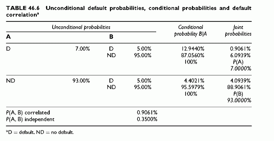
The process for calculating all the joint probabilities uses the conditional probabilities of Bs credit state given As credit state. In compact notation, P(A = D) = a designates the unconditional probability that A defaults and P(A = ND) = 1 — a the unconditional probability that A does not default, with similar notation for B [P(B = D) = b and P(B = ND) = 1 — b].
Three inputs determine all others: the unconditional default probabilities of A and B plus either the conditional probability that B defaults given A defaults, or alternatively the joint probability of default of A and B (using the simple formula applicable to two obligors as in Chapter 41). Table 46.6 shows the detailed calculations. The joint default probability P(A, B) results from the general formula:
Loss Distribution
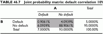
The process above results in the matrix of Table 46.7 cross-tabulating both entities credit states showing the joint probabilities, with the margins summarizing the column probabilities and the row probabilities, which equal the unconditional probabilities. This provides the loss distribution.
The same observation on single defaults applies to the independent and correlation cases. The single probabilities of default in a portfolio context differ from the unconditional probabilities of default. For instance, the default of A alone has a probability of
6.094%, whereas its unconditional default probability is 7%. How can we explain the paradox of differing single default probabilities of A out of a portfolio and within a portfolio? The explanation is that A defaulting alone, in a portfolio context, is conditional on others not defaulting and is no longer an unconditional probability of default. It is the joint probability of default of A and of others not defaulting.
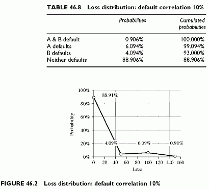
The standard presentations of the loss distribution, with cumulated probabilities, and the related graph are shown in Table 46.8 and Figure 46.2, respectively.
The Loss Statistics
The calculations show that the EL remains the same as with the independent case, as expected since expectation is not dependent on correlation. The LV and loss percentiles increase with the correlation (Table 46.9). These calculations allow us to relate the portfolio loss statistics to standalone risk measures, such as expected loss and loss volatility, and measure the effect of diversification.
The gain in LV quantifies the diversification effect: 36.412 — 27.744 = 8.668. Since risks do not add arithmetically, allocating the overall portfolio risk to each obligor is an issue. The risk contributions are risk allocations, dealt with in Chapters 51 and 52.
Comparisons of the Correlation and the Independent Cases
Correlation implies the following changes:
• The joint default probability is now higher than the product of the unconditional (standalone) default probabilities of A and B.
• The conditional default probabilities now differ from the unconditional (standalone) default probabilities.
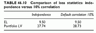
As a result, the distributions fat tails gets thicker and the distribution mode shifts to the left-hand side. This results from the higher probability of big losses (150). Table 46.10 shows that the portfolio EL remains the same while the LV increases with correlation. In addition, the probabilities of larger losses are larger, as expected, than in the independent case.
Analytical Loss Distributions
This chapter describes some analytical loss distributions when single defaults correlate with each other. The most developed model of analytical distributions is CreditRisk+. Other simple techniques allow us to simulate and visualize the effect of correlation on portfolio risk, measured by loss volatility and loss percentiles, under restrictive assumptions.
The starting point is the simple case of independent losses. The portfolio distribution of the number of defaults is the well-known binomial distribution. This is also a loss distribution applying to uniform (equal) exposures only, since the binomial distribution does not accommodate size discrepancies. The binomial distribution over a uniform portfolio serves as a benchmark for measuring the effect of correlations on the portfolio risk. It also illustrates how the increase in loss volatility, as a percentage of the total portfolio exposure, tends rapidly towards zero when increasing the number of obligors.
The limit distribution corresponds to another simple case with a uniform correlation between uniform exposures, building on a simplified version of the Merton model. To obtain closed-form formulas, we assume that the standardized asset values of firms follow normal distributions with a uniform correlation across firms. The uniform correlation results from the common dependence of all individual asset values on a single factor, representing the state of the economy. This single factor conditions the normal distributions of asset values. When conditions improve, all asset distributions shift upwards, resulting in a lower portfolio default probability than its unconditional long-term value. Conversely, when conditions worsen, the default probability of the portfolio becomes higher than its long-term value. In essence, the technique relies on conditioning the asset value distributions on a single factor. Additional simplifying assumptions allow us to obtain an analytical form of the portfolio value distribution, called the limit distribution. The limit distribution ignores specific risk. An important finding of such distributions, confirmed empirically by full-blown models, is that the fat tail of the loss distribution is highly sensitive to the correlation between defaults.
The next chapters (48 and 49) illustrating Monte Carlo simulations use a similar one-factor model to generate correlated defaults, accommodating unequal exposures and unequal default probabilities of individual obligors.
CreditRisk+ uses actuarial techniques to find the shape of the loss distribution in a more accomplished manner, using the Poisson distribution to model the number of defaults. Starting from independent defaults, CreditRisk+ models defaults using a mixed Poisson distribution. The critical parameter of this distribution is the default intensity per unit of time, analogous to a default probability. It applies only to independent defaults. The mixed Poisson distribution uses as default intensity the product of the long-term (unconditional) default intensity with a multiple called the mixing parameter. The technique accommodates mixing parameters dependent on common factors, resulting in correlated default intensities of the various banks portfolio segments.
The three sections of this chapter detail respectively: the binomial distribution; the limit distribution; the CreditRisk+ analytical framework.


