MODELLING JOINT MIGRATIONS AND DEFAULTS UNDER THE OPTION THEORETIC FRAMEWORK
Category: Risk Management in Banking
This section discusses joint migration probabilities within the option theoretic approach of default and migration. The drivers of credit risk are asset values and the level of debt. Credit risk events include default events and credit migration events. We discuss both sequentially. The principle of the technique is to model the joint probability of the assets of two obligors falling under thresholds triggering either default or migration events.
Correlation and Joint Default Probability
Default events occur whenever the asset value gets lower than the debt. The joint default of a pair of obligors occurs when both of them have asset values under the debt value. This joint probability embeds the correlation of default events. Asset values are uncertain and follow lognormal distributions. The normal distribution is acceptable as a proxy for practical purposes.
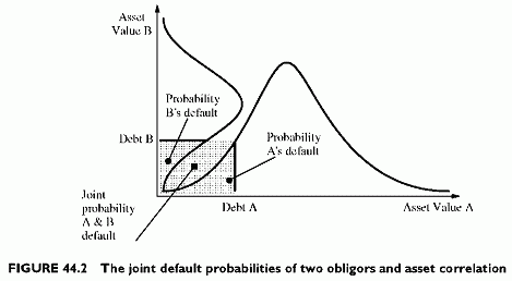
The joint probability of default is the area under the left and down rectangle between the origin of the axes and the two lines representing the debt levels of two obligors A and B in Figure 44.2. Both default when the asset value of A falls below its debt and when the same happens simultaneously to B. The area under the distribution curves visualizes these probabilities for A and for B. The figure shows different levels of debt and different values of expected asset values of A and B, as well as different volatilities.
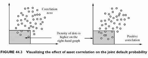
The correlation effect on the joint default probability appears in Figure 44.3. The figure plots the asset values of two obligors on two axes. The cloud of dots is more or less round according to correlation. With a zero correlation, the cloud of dots is a circle. When correlations increase, it tends to spread across the first diagonal. The density of dots in the rectangle represents the joint default probability. The rectangle does not change because it results from fixed values of the debts of A and B. With an elongated cloud of dots, the number of dots inside the rectangle changes, and this number of dots represents the frequency of joint defaults.
Credit Metrics derives the correlations from those of equity returns, using a multi-factor model. By contrast, KMV Portfolio Manager extracts the correlations from the modelled asset returns and uses a multi-factor model with orthogonal (independent) factors.
Correlation and Joint Default and Migration Probabilities
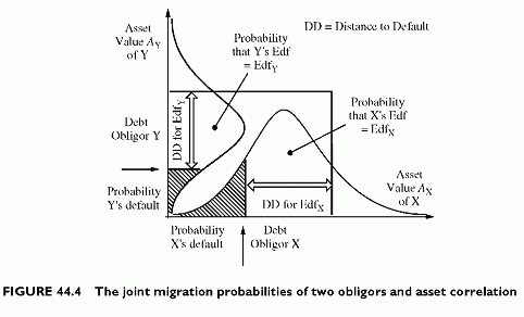
The same model applies to migration correlations derived from asset values. The same model of default correlation extends to correlations between migration events of two obligors. The only difference is that the thresholds driving the final rating differ from that of default. Now the thresholds are such that A gets the expected default frequency EdfA and B gets EdfB. Both thresholds are evidently above the default thresholds determined by the debt levels. Correlations determine the density of dots within the new larger rectangle. Asset correlations generate joint migration probabilities as they do for default events. Figure 44.4 uses a presentation similar to that of defaults. Credit Metrics models migrations using various threshold levels to define bands of asset values at the horizon defining the final risk classes.
Calculation of Joint Default Probabilities from the Distributions of Asset Values
In practice, the joint probability of AX and AY being under the default point depends on asset correlations and the distributions of X and Y random asset values, which are AX and AY, respectively. With the normal distribution, the Joint Normal Density (JND) function of the random variables AX and AY has an analytical form:
In the formula, ЈAX and ctAx refer to the expectation and standard deviation of X,and similar notations apply to Y. The correlation coefficient between asset values is pAXAY.
The correlation between asset values pAXAY differs from the correlation of discrete default or migration events pdefaultXY. If the standalone default probabilities and the default correlation are available, the simple formula for calculating joint default probabilities of discrete events for a borrower B and a guarantor G is, using the compact notation of Chapter 41:
Note the change in notation. The correlation p is not the correlation of asset values of X and Y, but the correlation between their default events. Similarly, b and g are now the default probabilities of obligors B and G. The same formula applies for joint migration probabilities, except that the probabilities P (X) and P (Y) are not the default probabilities of X and Y defaulting, but that of X migrating to a given credit state and Y migrating to another credit state. In this case, since there are many final credit states for each obligor, there are as many joint probabilities as there are pairs of final states. The unconditional migration probabilities P (X) and P (Y) are those of published migration matrices.
The simple standardized distance to default model helps to model migrations with unobservable asset values using:
• The assigned default probabilities, considering that they embed all relevant information.
• A correlation structure between asset values, given from factor models.
Correlations between credit events derive from modelled asset value correlations. Portfolio models simulate correlated asset returns to define the probabilities that two firms migrate jointly to default. For default probabilities equal to 2.5% and 1% respectively, the threshold values are —1.96 and —2.33 respectively with the standardized normal distribution. The process requires simulating standardized asset values and assigning a default value (1 for instance) whenever the simulated asset value falls below the threshold level. This technique serves to model portfolio losses for firms with preset default probabilities. Chapter 46 describes how to generate loss distributions from defaults for a portfolio using this technique for defining default, once the default probability is given. To obtain an analytical derivation of the joint distribution of asset returns, the standardized joint normal distribution applies. The formula above, providing the joint migration probability from the option model of default, simplifies when using standardized normal distributions since their means are 0 and their standard deviations are 1.The formulas require plugging in correlations of asset values as inputs.


