Business — Banking — Management — Marketing & Sales

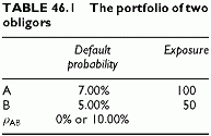
This section develops the case of a simple portfolio with two obligors A and B subject to correlated default risks. Table 46.1 describes the portfolio, with the unconditional (or standalone) default probabilities and the exposures of each. The loss given default is 100% of exposure.

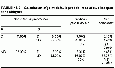
The loss distribution includes four points (values). The table provides the intermediate calculations of the corresponding probabilities. Correlation implies that conditional default probabilities now differ from unconditional default probabilities. In order to calculate the probabilities of the four possible loss values, we use the structure of conditional loss probabilities.

PORTFOLIO OF TWO INDEPENDENT OBLIGORS

The first case deals with independent defaults. In this simple case, all joint probabilities of any pair of credit states of A and B are simply the products of the unconditional probabilities of A and B having the corresponding credit states. A two-obligor portfolio might be a pair consisting of primary borrower+guarantor, or buyer of protection+seller of protection. The analysis illustrates the joint default probability of both entities (or double default probability), which is the unique default event for the lender. The calculations are similar to those detailed in the third-party guarantee analysis.

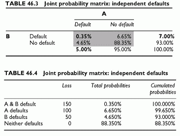
obligor within a portfolio. This is because, within the portfolio, the probability that only one obligor defaults is conditional upon non-default of the other, and hence different from the unconditional default probability. Finally, the example provides a general and simple framework to move from conditional probabilities, that are fairly intuitive, to correlations that are subject to less intuitive constraints (Tables 46.3 and 46.4, Figure 46.1).

The Loss Statistics

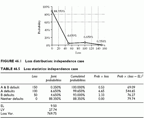
The calculation of the EL and LV follows directly from the probabilities of all joint events. The EL is the weighted average of losses, using probabilities as weights. The LV is the square root of the loss variance, which is the weighted average of the squares of deviation from EL, using joint probabilities as weights. Table 46.5 provides the intermediate calculations.

Finally, the loss percentiles derive from the cumulated probabilities. For instance, the loss percentile L(99.65%) = 100. The next lowest loss percentile is L(93%) = 50. There

is a 7% chance that losses exceed 50 and only a 0.35% chance that they exceed 100 (this is the joint default probability). When the confidence level is lower than or equal to 0.35%, the loss percentile is 150, for the double default of A and B.