REPORTING RISK AND PERFORMANCE MEASURES
Category: Risk Management in Banking
The basic risk measures used are:
• Exposure, either in value or as a percentage of total portfolio exposure.
• Capital in excess of expected loss, either in value or as a percentage of total portfolio capital.
• Edf as a percentage.
• Lgd as a percentage of exposure.
• Expected loss and unexpected loss.
• Income measures, either as spreads or risk-adjusted performance measures, namely the RaRoC ratio and SVA.
All dots in the sample charts of this chapter represent individual facilities. Subsequent sections provide sample reporting examples.
Facility Exposures and Risk Components (Edf and Lgd)
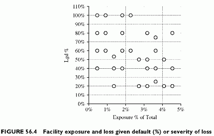
Two basic underlying components of credit risk, besides exposure, are the default probability (Edf) and the severity of loss under default, or loss given default (Lgd). They are basic ingredients of the expected loss EL, since Edf x Lgd measures the loss rate. In this sample portfolio, the default probabilities do not correlate with exposures. However, there are more small exposures in the area of high loss under default (low recovery rate). This is in line with expectations (Figure 56.4).
Setting Up Limits: EL and LV
Expected loss EL as a percentage of exposure is a relevant measure for risk quality, for assigning ratings or setting up limits and delegations. Loss volatility LV, both as a percentage of exposure and in value, synthesizes several risk dimensions, risk quantity, risk quality and capital allocation. Charts visualize the trade-off between risk quality and exposure.
Risk Quality versus Exposure
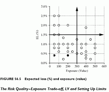
The EL-exposure graph (Figure 56.5) shows what happens when capping either EL or exposure. There are four quadrants, and points spread over all of them. The best measure of risk quality is EL as a percentage of exposure, while exposure (in value or as a percentage of total) measures the volume of risk. In addition, EL as a percentage is a frequent basis for rating risk because it combines both default probability and severity of loss. The EL in value serves better for economic provisioning. The EL as a percentage possibly serves for setting delegations and limits in terms of risk class. The graph shows EL as a percentage of exposure.
Capping exposure does not eliminate high EL, since there are many high ELs in the small exposure area of the chart. Conversely, capping percentage EL does not eliminate high exposures in general. The graph shows a tendency to take on more exposure for a small EL risk. It also shows that it is not equivalent to set a limit in EL and in exposure. Since exposure is not risk, because it does not embed all relevant risk dimensions, it is worth considering setting limits in EL.
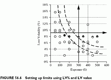
The LV(%)-exposure chart shows a similar picture (Figure 56.6). Since LV is the basis of capital allocation, capping LV is another option to up economic risk limits rather than exposure. Note, however, that EL and LV depend on the same risk components—EaD, DP and Lgd—although LV is closer to capital than EL.
The graph of LV(%)-exposure value also shows the trade-off between risk quality (EL% or LV%) and risk quantity (exposure). The product LV(%) x exposure is the LV in value. Bounding this product is similar to bounding LV in value. The various levels of LV value in the LV(%)-exposure graphs are hyperboles, each one corresponding to an LV value. Pushing the curve towards the centre limits both quality and quantity of risk. Lets assume that the lower curve shown in the graph is the limit. There are still several points above this curve. The implication is that the subjective trade-off between risk quality and risk quantity does not filter high LV values.
Risk-based limits in LV eliminate some small and large exposures that appear less risky than they are. In order to push the LV value under a preset limit, we have to decrease either the risk quality (EL% or LV%) or the risk quantity (exposure), or both, to move below the risk limit curve. Since LV relates to capital allocation, bounding the LV is a proxy for bounding economic capital allocation.
Risk-adjusted Performance and Mispricing Reports
The performance measures relate revenues to exposure or economic risk measures. Revenues are All-In Spreads (AISs), including interest margins and fees annualized over the life of the facility, either in value or as a percentage of exposure. The percentage measure is the accounting Return On Assets (ROA), which is not risk-adjusted because it relates revenues to the volume on risk only, ignoring risk quality.
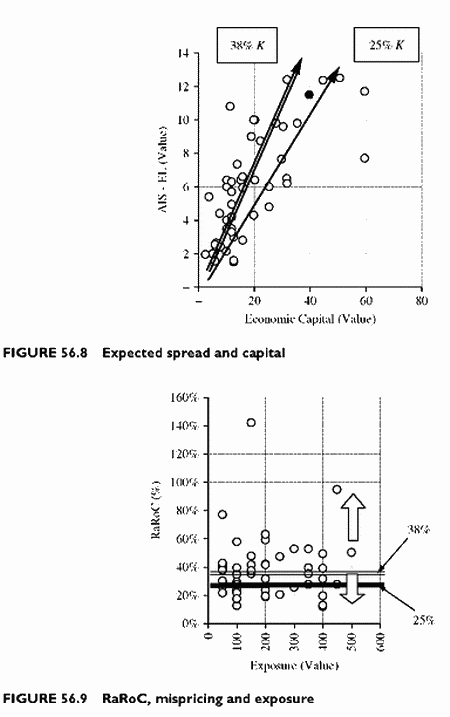
The risk-adjusted return is the RaRoC, or Sharpe ratio, of the facility, based on the allocated capital: RaRoC = (AIS — EL)/(allocated capital — EL). The RaRoC should be above the hurdle rate k, representing the target pre-tax and pre-operating expenses return on economic capital. RaRoC can be negative since it is the ratio of a difference in spreads and expected loss to allocated capital. The SVA is AIS — EL — kK. The SVA measure combines both size of transactions and risk-adjusted return. It shows the relative richness of transactions in value: positive SVA indicates creation of value. Unlike negative RaRoC, negative SVA has an interpretation, since it means destruction of value. The SVA minimum line is therefore the zero value horizontal line, a function of the 25% hurdle rate. The average SVA is the ratio of total SVA by the number of exposures, 50, or 1.24.
Risk-return profiles are also mispricing reports since they show gaps between target and effective pricing. Mispricing reports serve to identify which facilities contribute to the richness of the portfolio and which do not. There are two mispricing reports:
• The first mispricing is the gap between the target minimum return and the effective return. For RaRoC, the benchmark is the hurdle rate 25%. For SVA, it is the zero value showing that a facility breaks even on the cost of risk.
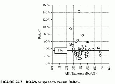
• The second mispricing is relative to portfolio average. It shows whether a facility is more or less profitable, after risk adjustment, to the average portfolio risk-adjusted return. For the RaRoC, the reference value is 38%.
For SVA, it is possible to use the average SVA as a benchmark, or 1.24. However, the SVA depends on size, so that the actual reference value for the portfolio should be the SVA per unit of exposure, or 61.82/11 000 = 0.56%. Mispricing would become the gap between the SVA per unit of exposure for each facility and the portfolio average unit exposure SVA.
We provide below representative reports for our sample portfolio (for illustration only).
RaRoC Reports
Figure 56.7 shows that accounting measures of profitability (ROA%) and risk-adjusted measures (RaRoC%) have no relationship. This is the primary reason for risk-adjusting performance measures. Negative RaRoCs appear in real portfolios whenever the spread does not compensate the EL plus allocated costs. When isolating a transaction, the AIS might not exceed EL because market spreads might not compensate risk. The phenomenon often disappears when extending revenues to all transactions and services to a client, because fees and other profitable transactions might more than compensate the lowest profitability transactions originated to build up business volume with a client.
AIS — EL in value plotted against capital shows the numerator and the denominator of the RaRoC ratio (Figure 56.8). All points above the 25% line create values and all points below the line destroy values. All points above the 38% line are richer than the portfolio average, and conversely. Mispricings are gaps between the points and the two lines representing 25% x K and 38% x K. The graph shows both what the pricing should be (in terms of risk-adjusted return) and what it is effectively. It also allows us to identify over- and underpriced facilities compared with either the hurdle rate or the average return.
The plot of RaRoC versus exposure provides another view of mispricing (Figure 56.9). It shows which facilities are above the 25% hurdle rate. All points above the horizontal 25% line create values, and all points below destroy values. Similarly, all points above the 38% average contribute to increasing the portfolio RaRoC above the average, and vice versa.
SVA Reports
The SVA reports are in value (Figure 56.10). The graphs compare each facility SVA with the arithmetic average of the portfolio. This is convenient, but not accurate, since the SVA combines both size and profitability. An alternative graph would show the unit exposure SVA of each facility and compare it with the average unit exposure SVA of the portfolio. In any case, there are negative SVAs, which correspond to RaRoC points lower than the 25% hurdle rate. The 25% RaRoC value corresponds here to the zero SVA value.

