SIMULATIONS BASED ON ECONOMETRIC MODELS
Category: Risk Management in Banking
A summarized description of a simplified econometric structure serves to define the simulation framework. After making explicit the set of simplifying assumptions, we present simulations for a two-segment portfolio.
Econometric Modelling Structure
CPV models the default and migration rates of portfolio segments as a function of explicit economic indexes, and allows us to capture the cyclical dynamics of industry-country factors. As a reminder, the CPV structure uses two basic blocks:
• Type 1 models provide the default rates of each segment DR,- (N segments) as a logit function of an economic index Y{. There are as many indexes Y{ as there are segments, or N. Each index Y, depends on multiple economic factors X,- (K factors). There are N models for the N segments. Hence, there are N residuals.
• Type 2 models provide the predicted values of the K economic factors X, using an Auto Regressive Integrated Moving Average (ARIMA) fit. There are K economic factors. Hence, there are K models and K new residuals.
To generate a distribution of portfolio values, CPV uses Monte Carlo simulations of the factors influencing the default and migration rates of segments. Due to the dependence on common factors, these simulated rates correlate. The process requires:
• Simulating the predicted values of each factor influencing the index, on which default rates depend, from past values and error terms using time series modelling.
• Simulating the predicted values of segment default rates from the simulated values of the indexes influencing them, the simulated values being generated in the first step above from simulation of future values of country-industry factors.
We use t as the current date and t + 1 as the horizon value, by definition a future date when all factors and default rates become random as of today. The three types of equations
Given the modelling structure, the simulation technique is complex.
We know that within each model, whether logit or ARIMA, the error terms are independent of the explanatory variables. When looking forward (date t + 1), taking as given thevaluesasofdate t, we generate random values as of date t + 1 using the residuals of each model. Each residual has a zero mean and a standard deviation resulting from fitting the model. But the residuals of the different models have no reason to be independent. In general, they correlate. Therefore, we need to generate random values of residuals, of all equations, that comply with their correlation structure. Random values of country-industry indexes conditional on past values of factors and errors result from simulating correlated values of the error term ek; i+1.There are K factors and K residuals ek,t+1. Once this set of correlated predicted values of country-industry factors Xk,t+1 is generated, we need to infer the values of the indexes YЎ, t+1 by generating random values of the error terms of the fits of indexes to factors, eЎ; t+1.There are N segments and N residuals eЎ,t+1. Since there are also cross-correlations between the residuals ek;t+1 and eЎ;t+1, we need to perform this step in conjunction with the generation of predicted values of factors, in order to preserve both correlations between factor error terms and cross-correlations with index error terms. Finally, the default rate simulated values result from the logit function for all segments. They correlate because they depend on common factors and because of the correlation of the cross-correlation of residuals (Figure 48.5).
The long-term transition matrix serves as the unconditional migration matrix. Short-run migration matrices are conditional on the state of the economy, or default rates. They need to comply with internal consistency constraints since all migration rates have to sum to 1 after adding the default rate for each risk class. They also need to comply with external consistency constraints such as the lower volatility of default rates for investment grade ratings.
The CPV open framework allows customization to any observable data set, but requires modelling as a prerequisite. In addition, it provides an explicit link with the economic cycle dynamics, using observable factors. By contrast, KMV provides the proprietary model bundled in the package, but the interpretation of the axes driving the risk concentrations of the portfolio is not straightforward.
The Simplified Model
We proceed by conducting a sample simulation using, as usual, a much simpler framework. There are two portfolio segments and only one factor driving the index, converted into
segment default rates through the logit function. We detail the simpliied structure of modelling before providing sample simulations.
The Structure
We use a one-factor model for the index Y{; t+1, serving as an argument in the logit function to calculate the default rate. There are two portfolio segments 1 and 2, and i = 1 or 2. The single common factor Xt+1 influencing all segment indexes follows a standardized normal distribution. This allows us to omit the k of Xk,t+i. Using one factor directly driving the default rates through Y{, t+1 bypasses the time series model of CPV, which makes this index dependent on past values of other factors and error terms from ARIMA fits. There is no need either to worry about the correlation structure of the multiple error terms of ARIMA models. The index ,t+1 is a linear function of the X t+1 and includes an error term e{, t+1 as well, independent of the X t+1 factor. Generating random values of this error term is equivalent to generating correlated random values of the Yj,t+1 converted into correlated default rates of segments. In addition, we assume that the correlation p between the index , t+1 and the unique factor X t+1 is common to the two segments. This is only a convenient simplification. Finally, the model operates in default mode only, without revaluation according to the final credit state. This bypasses the transition matrix modelling and the revaluation block.
The Model
There is a single Xt+1 factor for the two segments 1 and 2 for default rates indexed DR, with i being 1 or 2. The two portfolio segments 1 and 2 have different mean default rates. They represent, for example, two industries whose risk classes differ on average. The default rate DR, of each segment depends on two economic indexes Yf,t+1. Both indexes Y1;t+1 and Y2;t+1 depend on one common factor Xt+1 that correlates them. Each industry index is random and drives the corresponding segment default rate through the logit
Sample Simulations with Correlated Default Rates
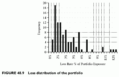
Figures 48.6 and 48.7 show the frequency distributions of the default rates of segments 1 and 2. The distributions of the default rates are highly skewed to the right. It is visible from the frequency distributions that the average value of the default rate of segment 1 is lower than that of segment 2. The scatter plot of one default rate against the other shows how correlated their values are (Figure 48.8). Finally, the loss distribution of the portfolio aggregates the correlated distribution of default rates of the two segments.
The default rates, with a 40% correlation of factor values, have a correlation of 44%. This is visible in the scatter plot of the two sets of values.
Table 48.2 summarizes the statistics of the simulated default rates and those of the loss rate for the portfolio. The loss distribution presents the characteristic skew to the
right. The values are weighted averages of pairs of default rate values generated by each simulation run. The frequency is a percentage of the number of obligors. The loss rate peaks, in this simulation, at 12.5%. The peak is lower than the peak values of the segment default rates, because they do not reach their peak values at the same time, so that the overall loss rate average value is lower than the average of the peak values of 1 and 2 default rates. Using a lower correlation between factors driving the default rates would result in a shorter fat tail.
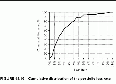
From this loss distribution (Figure 48.9), we derive the cumulated loss distribution (Figure 48.10). This is the cumulated frequency of having values lower than the X-axis
percentage. The cumulative distribution visualizes the loss percentiles. For instance, the peak loss in the simulation is 12.5%. The 97.5% loss percentile is 11% and the 95% loss percentile is 10% of the overall loss rate.
Although this is not a comprehensive description of CPV, it illustrates the CPV modelling philosophy. With a simple framework, the technique appears straightforward. In practice, there are difficulties due to the scarcity of data on default rates. If observations are yearly, it is difficult to imagine more than 30 observations. In addition, a long period might make it less relevant for todays measures. Finally, even though CPV provides a comprehensive framework, it lets end-users make the final choices. In spite of these constraints, CPV is the sole model capturing explicitly the cyclical dynamics of default rates.
Loss Distribution and Transition Matrices
This chapter explains how to derive distributions of the portfolio values using joint migration matrices. The principle is to find all final risk classes of each firm within the portfolio. The revaluation of assets at the horizon uses the final credit spread that applies to each final risk class. The distribution of portfolio values results from the individual distribution of all states for each facility.
The joint migration matrices determine all possible combinations of migrations of two obligors and assign joint probabilities to each of them. Now, we move one step further, combining joint migration probabilities with revaluation to obtain the loss distribution.
This chapter uses the simple matrix calculated in Chapter 28 to show how to obtain the portfolio value distribution. The first section discusses the joint migration matrix example and the second derives a value distribution for a simple portfolio of two obligors.


