Business — Banking — Management — Marketing & Sales

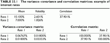
The assumptions of the Delta VaR technique make it analytical, using closed-form formulas for determining loss percentiles. Since there are as many covariances and correlations as there are pairs of random variables, it is convenient to group these statistics in matrices. The matrices cross-tabulate the variables in rows and columns. The covariance, or the correlation coefficient, is at the intersection of the row and the column relative to this pair of variables. Since both correlations and covariances do not depend on the sequence of the two variables, the matrix is symmetric around its diagonal. Along the diagonal, the values are the variances of each variable since they are the covariances of each variable with itself. Any variance-covariance matrix needs to comply with such properties. In this example, no specific risk term appears because we use deterministic relationships between two interest rate exposures and the corresponding rates. When there is a specific risk, it is necessary to add to the portfolio volatility all specific risk error volatilities as well as the general risk, since the specific risks are independent of the factors driving general risk.

Example of a Variance-Covariance Matrix

The statistics of the above example correspond to the 2 x 2 matrices in Table 32.1.

Calculation of the Loss Volatility

We calculate the variance and the volatility of a portfolio of two interest rate exposures using a sample set of data. These are market exposures. The same process would apply to mark-to-market values of loans sensitive to interest rate variations. We need to specify the exposures. In order to make explicit calculations, we need to use the property of expectations and volatility when we multiply exposures (certain) with a random variable as in the first section.

Direct Calculation of the Two Exposures Portfolio Volatility

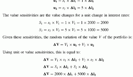
The example is a portfolio of two market exposures to interest rates with zero-coupon bonds of maturities 1 and 5. The sensitivities³ are 1 and 5. There is a positive correlation between the interest rates for 1 and 5 years. The current market values are 2000 and 1000, with a total portfolio value of 3000. The value sensitivities for a unit change in market rates are 1000 and 5000. It is convenient to define the random value change for a unit size exposure, or return. These unit random losses are the percentage sensitivities, 1 and 5, times the random changes of interest rates, Aii and Ai₂, of the two interest rates. Unit random returns:

The volatility of the portfolio value is the volatility of this sum of random changes of two interest rates, weighted by sensitivities considered as certain:

This direct calculation extends to any number of exposures and market parameters. The matrix format makes the process simple.