Business — Banking — Management — Marketing & Sales

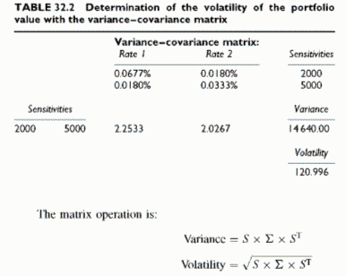
The matrix format helps when using a general formula applying to any number of exposures. The starting point is the sensitivity vector of individual exposures. The variance-covariance matrix summarizes the interdependence between the entire set of market parameters. Using the above example, the portfolio volatility is the row vector of sensitivities multiplied by the variance-covariance matrix, times the column vector of sensitivities. The example uses value sensitivities. The intermediate steps of the calculation are identical to the above calculations. The matrix format of Table 32.2 summarizes them.

where S is the row vector of value sensitivities, S^T is the transposed vector and £ is the variance-covariance matrix of all market parameters.

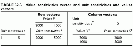
Note that unit sensitivities necessitate a slightly different format (Table 32.3). The value sensitivity S is the percentage sensitivity times the value. Hence, the vector S is the product of the row vector of unit sensitivities times the row vector of values. The transposed vector S^T is the transposed product⁵: S = sV and S^T = (Vs)^T = V^Ts^T.The variance matrix formula becomes: Variance = sV x £ x (sV)^T.

The resulting volatility from the example in Table 32.3 is 121 rounded. The same matrix formulas serve for any number of exposures, as long as we stick to the constant sensitivities as a proxy of reality. This concise format serves both for market risk VaR, where volatility is important, and for credit risk VaR, since the portfolio loss volatility is also an important parameter.

For credit risk, the same methodology uses the values of exposures to credit risk to obtain the loss volatility, rather than the value sensitivities as above.

Summary of the Delta-Normal Technique

Figure 32.5 summarizes the methodology. A matrix operation provides the portfolio variance and volatility, using the vector of sensitivities and the variance-covariance matrix:

When there is specific risk, the variance sums the general risk volatility, as derived from sensitivities and the variance-covariance matrix, and the specific risk terms. The variance-covariance matrix embeds these terms in the diagonal, as the diagonal applied to stocks demonstrates. The difference is that the sensitivities do not suffice for capturing total risk, whereas they do in the case of deterministic relationships between individual

risk and market parameters. Since the portfolio value at the horizon is normal, the problem is to find the volatility of the market value of the portfolio in order to derive the VaR. The volatility formula combines the sensitivity vector with a variance-covariance matrix. Then, VaR results from simple multiples of the normal distribution mapped to conidence levels. In the formula, it is easy to use value sensitivities, as in the example below. There is no need for simulations, since we use a closed-form expression for portfolio value volatility.

With the above example, the yearly volatility is rounded to 121. The 1% one-tail confidence level is 2.33 for a normal distribution. This would result in a yearly VaR of:

This yearly volatility has to be converted to fit the shorter period required for market risk VaR, that is 10 days. The simplest conversion rule uses the square root of time coefficient since the period considered for market risk is very short. The 10-day volatility is VW250 = V0.04 = 0.2 times the yearly volatility 121. Since the VaR is proportional to volatility, the same coefficient applies to obtain the 10-day VaR. With a yearly VaR of 291, we multiply it by 0.2 to get the 10-day VaR, or 0.2 x 237 = 56.40⁶.

The regulator allows the usage of proprietary models for calculating VaR and economic capital. The quantitative requirements are: a one-tailed confidence level of 99%; a 10-day holding period; observation periods of at least 1 year, with periodical quarterly updates as a minimum; a multiplication factor of 3, possibly adjusted. The multiple covers extreme events, errors, lack of liquidity of markets and of exotic instruments, long periods of adverse market movements. The VaR is the maximum of the last daily VaR and the last 60-day average. The multiple is subject to variations depending on the reliability of the VaR measures, as assessed through back testing. This provides a feedback loop after back testing as well as an incentive to refine the methodology.