Business — Banking — Management — Marketing & Sales

Delta VaR makes the individual returns a linear function of market parameter returns. The Delta-normal VaR technique assumes normality of returns distributions, resulting in a normal distribution of the portfolio returns. The volatility of the portfolio return uses the general formula that applies to any set of linear combinations of random variables. Since we can calculate the volatility of the portfolio return and since we know that it is normally distributed, we have all that we need for measuring VaR. The shape of the normal distribution depends on correlations across market parameters. However, the expectation and the volatility suffice to determine the normal distribution of the portfolio return and to derive all loss percentiles and market risk VaR. Since the process does not require any simulation, it is an analytical technique with simple calculations of VaR. The Delta VaR technique contrasts with simulations that generate the portfolio return distribution, and derive empirically from its shape the various loss statistics of interest.

Portfolio Value as a Function of the Set of Market Parameters

The asset returns are a linear function of market parameter changes. Since all assets within the trading portfolio depend on various subsets of the global set of market parameters, its value relates to them through sensitivities as well. The portfolio sensitivities are linear combinations of the various individual transaction sensitivities. When modelling portfolio return, we obtain the AV_p/V_p0 and derive directly AV_p results from the known current value V_p0. The formula also includes the specific risk terms when sensitivities capture only a fraction of asset returns (such as for stock return):

The indices are k (1 to K) for the market parameters and i (1 to N) for the individual transactions. The double summation, first over all transactions, then over all market parameters, results from the fact that any single transaction is a function of a subset of the K market parameters. Since the portfolio includes all transactions, and since all of them depend on various market parameters, the portfolio is sensitive to all market parameter changes. It is convenient to introduce the portfolio sensitivities S_pk, which are linear combinations of single transaction sensitivities:

This is a linear relationship between the portfolio value return y_p and the market parameter returns as long as the sensitivities are constant. Since returns are normally distributed,

the value changes are (1 + y_p) x V₀ and are normally distributed as well. However, the volatility of the normal distribution of the portfolio value at the horizon depends on the entire variance-covariance structure of the market parameters.

The Portfolio Value Distribution

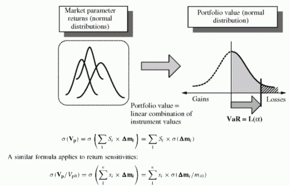
The next step is to derive from the linear model the distribution of the portfolio value given the distribution of the individual market parameters. Using normal returns results in a normal distribution. This normal distribution embeds all correlations since the process uses correlated market parameter returns¹. A linear combination of normally distributed variables also follows a normal distribution, whose expectation and volatility derive from the individual distributions and their variance-covariance matrix. This makes it easy to characterize the portfolio distribution as a function of the market parameters selected for mapping the instrument values and the sensitivities of individual asset returns (Figure 32.4).

FIGURE 32.4   From instrument value distributions to portfolio value distribution

We can use return sensitivities or value sensitivities. The volatility of the variation of the portfolio value is the volatility of a sum of random individual changes weighted by sensitivities:

The derivation of this volatility results from the variance formula for a sum of random variables. The details of this calculation are in the example below. Using the distribution of AV_p allows us to define any loss percentiles along the normal distribution. The VaR is a loss percentile L(a) with a given confidence level a. Mapping loss percentiles with multiples of the normal distribution volatility uses the well-known multiples of volatility. Figure 32.4 illustrates the process.