Business — Banking — Management — Marketing & Sales

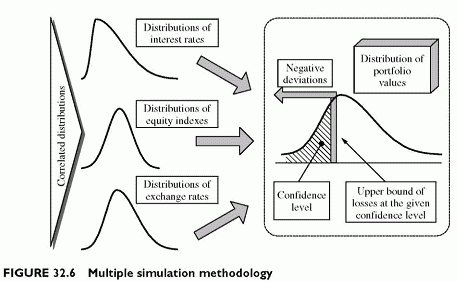
The principle of the simulation method is to test multiple possible outcomes against a portfolio to obtain its risk. A set of future values of market parameters characterizes each scenario. These future values result from time path simulations of their returns if necessary. Each set of parameter values serves for revaluing the portfolio. The revaluation process uses pricers, models for valuing instruments and sensitivities for stock prices. By generating a large number of such scenarios, it is possible to generate a large sample of portfolio values. From this distribution of portfolio values, we derive empirically both the volatility of market deviations and the upper bound at a given confidence level.

Principle of Multiple Simulations

The multiple simulation methodology is empirical. There is no need to make assumptions about the shape of portfolio value distributions. This shape results from mechanical revaluations of the portfolio for all runs of market parameters. Then, the determination of the bound for losses is empirical, or non-parametric (Figure 32.6).

When the linear approximation collapses, as for options, and when we cannot use shortcuts to approximate final values, we need to revert to the full valuation technique. This implies simulating risk drivers, eventually using their entire time path, and obtaining their final values and pricing models for some standard derivatives. The direct revaluation bypasses the proxy formulas using sensitivities, but it makes the process more calculation intensive. Forward revaluation of derivatives might need simulations beyond the horizon, starting from each possible value at the horizon, or simulations within simulations, making the process overly complex.

Because of these complexities, several techniques help to simplify the process. One way to address the calculation intensive process is to minimize the number of simulations¹¹. There are several variations around these common principles. We review the simplest ones, before addressing the full-blown simulation process. They include:

• Grid simulations.

• Historical simulations.

Full Monte Carlo simulations.

Grid Simulations

Before generating a very large number of scenarios it is tempting, in order to limit the calculations, to restrict the approach to a small number of scenarios. The grid Monte Carlo approach uses an exact valuation for each grid point and uses a linear interpolation between points.

Grid simulation consists of running a limited number of sets of parameter values. The selected values should cover a maximum range of values of each parameter. Since there is a limited set of values, the process is less calculation intensive than full Monte Carlo simulations that aim for a comprehensive coverage of possible market outcomes. For instance, it is possible to focus on shocks of various parameters to try to capture all main deviations from current value of the portfolio. This is not as powerful as full-blown simulations, because the selection of values might miss some worst-case scenarios.

Some techniques attempt to identify these worst-case situations empirically. As a reminder, it is not feasible to identify worst-case scenarios with a large variety of exposures because of offsetting effects. Stressing one parameter might increase the overall loss. However, for some instruments it generates adverse deviations and for others gains. Therefore, it is possible that a different shock will capture another worst-case situation that is even worse than the previous one. A practical way of identifying such worst-case scenarios is to examine the portfolio structure, to identify its main exposures and their risk drivers, and to try several shocks on various parameters driving the risk of the major exposures. Then, some scenarios will prove worse than others, and selected scenarios for stressing the loss of value of the portfolio could be sampled from this set.